Week 5: All Roads Lead to Rome#
Hello everyone, time for another weekly blogpost! Today, we will talk about taking different paths to reach your objective.
Last Week’s Effort#
After having the FBO properly set up, the plan was to finally render something to it. Well, I wished for a less bumpy road at my last blogpost but as in this project things apparently tend to go wrong, of course the same happened with this step.
Where the Problem Was#
Days passed without anything being rendered to the FBO. The setup I was working on followed the simplest OpenGL pipeline of rendering to an FBO:
Setup the FBO
Attach a texture to it’s color attachment
Setup the shader to be used in the FBO render and the shader to render the FBO’s Color Attachment
Render to the FBO
Use the color attachment as texture attached to a billboard to render what was on the screen
But it seems like this pipeline doesn’t translate well into VTK. I paired again on wednesday with my mentors, Bruno and Filipi, to try to figure out where the problem was, but after hours we could not find it. Wednesday passed and then thursday came, and with thursday, a solution: Bruno didn’t give up on the idea and dug deep on VTK’s documentation until he found a workaround to do what we wanted, that was retrieving a texture from what was rendered to the screen and pass it as a texture to render to the billboard. To do it, he figured out we needed to use a different class, vtkWindowToImageFilter, a class that has the specific job of doing exactly what I described above. Below, the steps to do it:
windowToImageFilter = vtk.vtkWindowToImageFilter()
windowToImageFilter.SetInput(scene.GetRenderWindow())
windowToImageFilter.Update()

texture = vtk.vtkTexture()
texture.SetInputConnection(windowToImageFilter.GetOutputPort())

# Bind the framebuffer texture to the desired actor
actor.SetTexture(texture)
This is enough to bind to the desired actor a texture that corresponds to what was prior rendered to the screen.
This Week’s Goals#
Having a solution to that, now its time to finally render some KDE’s! This week’s plans involve implementing the first version of a KDE calculation. For anyone interested in understanding what a Kernel Density Estimation is, here is a brief summary from this Wikipedia page:
In statistics, kernel density estimation (KDE) is the application of kernel smoothing for probability density estimation, i.e., a non-parametric method to estimate the probability density function of a random variable based on kernels as weights. KDE answers a fundamental data smoothing problem where inferences about the population are made, based on a finite data sample. In some fields such as signal processing and econometrics it is also termed the Parzen–Rosenblatt window method, after Emanuel Parzen and Murray Rosenblatt, who are usually credited with independently creating it in its current form. One of the famous applications of kernel density estimation is in estimating the class-conditional marginal densities of data when using a naive Bayes classifier, which can improve its prediction accuracy.
This complicated sentence can be translated into the below image:
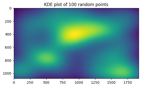
That is what a KDE plot of 100 random points looks like. The greener the area, the greater the density of points. The plan is to implement something like that with the tools we now have available.
Let’s get to work!